Bearing Fault Detection - Predictive Maintenance and Machine Learning Project
Project to detect bearing faults with 100% accuracy using CWRU vibration data with FFT signal processing and Random Forest machine learning.

⚙️ PREDICTIVE MAINTENANCE PROJECT
Bearing Fault Detection and Classification
Predictive Maintenance with FFT Signal Processing and Random Forest Machine Learning
|
%100
accuracy
|
12kHz
sampling
|
FFT
Signal Analysis
|
R.F.
Random Forest
|
1.1 General Purpose of the Project
The running parts (bearings, transmissions, etc.) of vehicles used in the defense industry and heavy industry conditions need to be analyzed in terms of sustainability. Using sensor data instead of traditional maintenance methods condition-based predictive maintenance (Predictive Maintenance) is planned to be done.
📊 Data SourceCase Western Reserve University (CWRU) laboratory data |
🎯 TargetPre-detection and classification of the fault |
2.1 Signal Processing and Frequency Analysis Phase
During the analysis phase, data obtained from the CWRU website 12k Drive End data was used. For analysis and processing of signals Python programming language was used.
Data Loading
Uploading data to the system and drawing time-dependent graphs.
Time Series Analysis
Defective bearing blows It was observed that .
FFT (Fast Fourier Transform)
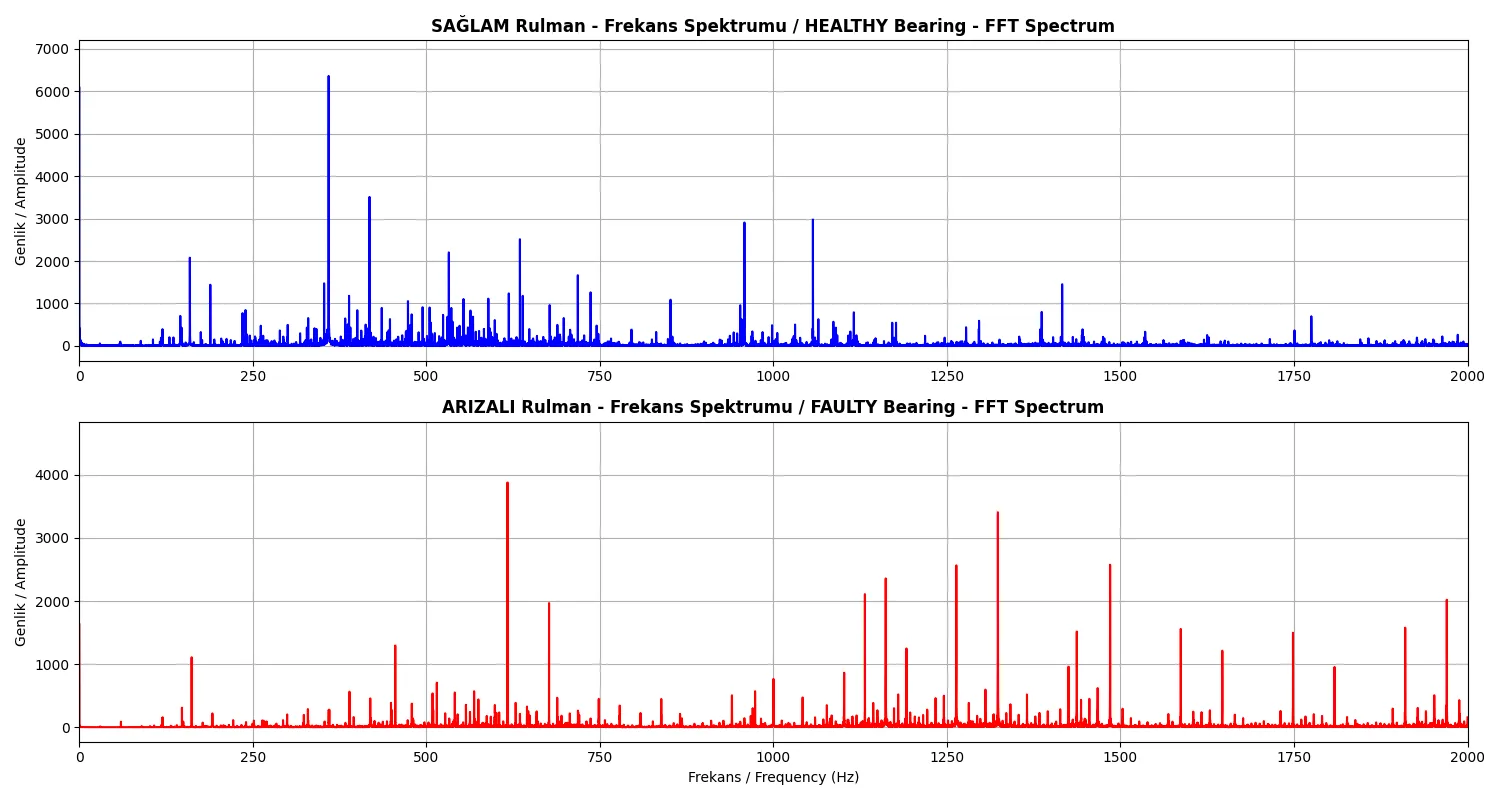
FFT process was applied to the signals to find the frequency of the pulses. In case of faulty signal around 160 Hz An increase in energy was detected.
✅ Result: It has been seen that these frequencies coincide with theoretical calculations.
💻 Signal Processing Code
# Source - https://stackoverflow.com/q (Modified by Community, CC BY-SA 4.0)

import scipy.io
import matplotlib.pyplot as plt
import numpy as np
from scipy.fft import fft, fftfreq

# Dataları yükleme kısmı
mat = scipy.io.loadmat('arizali.mat')
sinyal = mat['X105_DE_time'].reshape(-1)

# Perform FFT with SciPy
N = len(sinyal)
fs = 12000
yf = fft(sinyal)
xf = fftfreq(N, 1/fs)

# Pozitif frekansları alma
idx_max = N // 2

# Grafik Çizimi
plt.figure(figsize=(10, 6))
plt.plot(xf[:idx_max], np.abs(yf[:idx_max]))
plt.title('Arızalı Rulman Frekans Spektrumu')
plt.grid()
plt.show()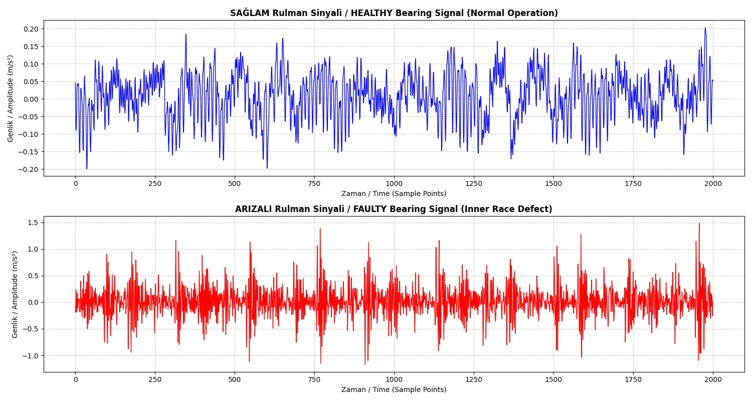
📊Figure 1 - Time Series Analysis | Figure 2 - Frequency Spectrum
3.1 Feature Extraction and Artificial Intelligence Application
Since direct analysis of raw signals is difficult, feature extraction It was decided to do so. signals into pieces of 1000 The following attributes were calculated for each part:
| attribute | formula | Description |
|---|---|---|
| RMS | √(mean(x²)) |
Effective value of the signal |
| kurtosis | scipy.stats.kurtosis() |
The sharpness measure of the distribution |
| Max Value | max(|x|) |
Maximum absolute value |
📊 Observation: It is seen in the graph that healthy and faulty data are separated from each other when calculated based on RMS values.
💻 Feature Extraction Code
# Source - StackOverflow (CC BY-SA 4.0)
import pandas as pd
from scipy.stats import kurtosis

def ozellik_cikar(sinyal, etiket):
    ozellikler = []
    parca_boyutu = 1000
    for i in range(0, len(sinyal) - parca_boyutu, parca_boyutu):
        parca = sinyal[i : i + parca_boyutu]

        # RMS ve diğer özellikler hesaplanıyor
        rms = np.sqrt(np.mean(parca**2))
        kurt = kurtosis(parca)
        max_val = np.max(np.abs(parca))

        ozellikler.append([rms, max_val, kurt, etiket])
    return ozellikler

# DataFrame oluşturma
df_features = pd.DataFrame(ozellikler,
    columns=['RMS', 'Max_Value', 'Kurtosis', 'Label'])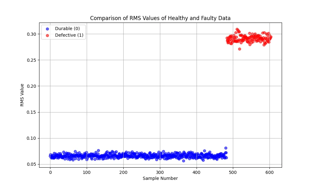
📊Figure 3 - Feature Separation (RMS)
4.1 Evaluation of Results
Obtained attribute data Random Forest It was trained using the algorithm.
|
%100
Accuracy
|
80/20
Training/Test Ratio
|
📈 Feature Importance: Your most important feature Maximum Value and RMS It was seen as a result of the analysis.
🔍 Confusion Matrix Results
Model intact and defective parts without error has separated.
💻 Model Training Code
# Source - StackOverflow (CC BY-SA 4.0)
from sklearn.ensemble import RandomForestClassifier
from sklearn.metrics import accuracy_score
from sklearn.model_selection import train_test_split

# Split Data
X = df_features[['RMS', 'Max_Value', 'Kurtosis']]
y = df_features['Label']
X_train, X_test, y_train, y_test = train_test_split(
    X, y, test_size=0.2, random_state=42)

# Model Training
model = RandomForestClassifier(n_estimators=100)
model.fit(X_train, y_train)

# Prediction
y_pred = model.predict(X_test)
acc = accuracy_score(y_test, y_pred)
print(f"Model Accuracy: {acc*100:.2f}")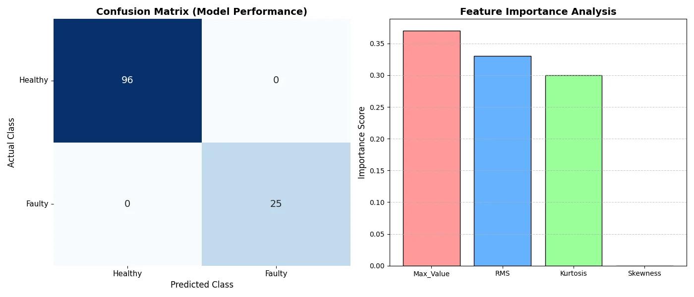
📊Figure 4 - Confusion Matrix
🛠️ Technologies Used
|
🐍
Python |
📊
NumPy |
🔬
SciPy |
🤖
scikit-learn |
📈
matplotlib |
🐼
pandas |
Related Projects
View All ->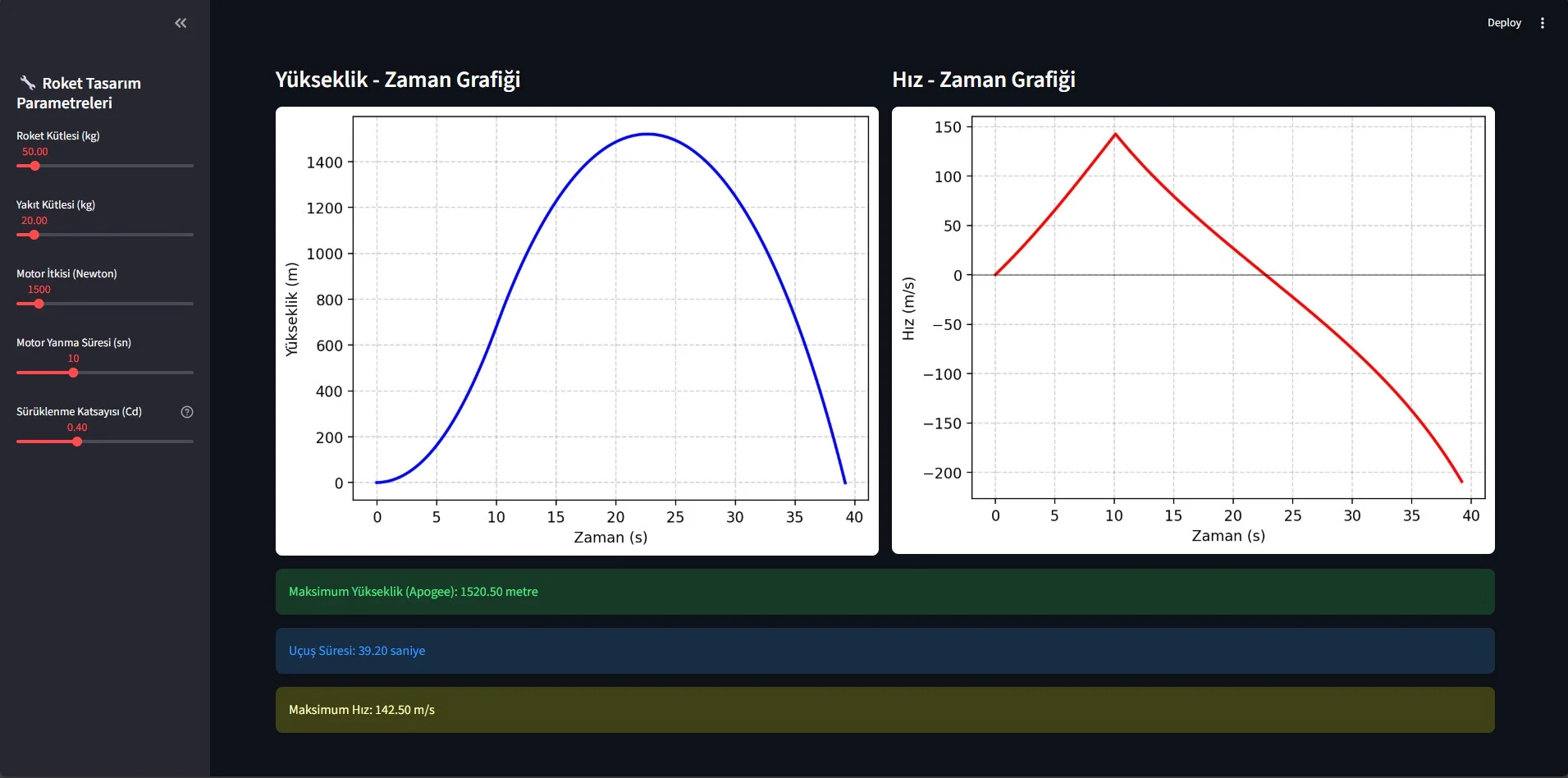
SkyTrace - Python Based Rocket Orbital Simulation
Parametric rocket simulation developed with Newton's laws of motion and aerodynamic drag principles....
View Project arrow_right_alt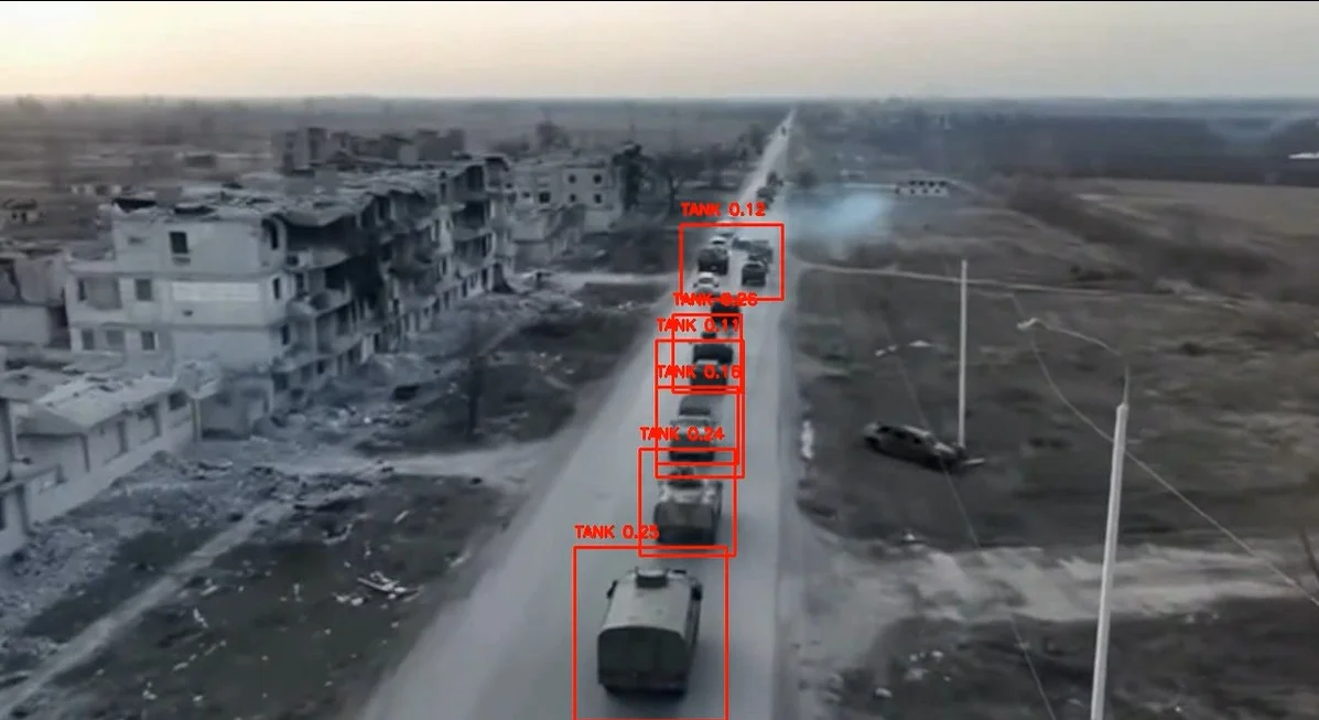
Real-Time Tank and Armored Vehicle Detection with Spotter UAV-YOLOv8
YOLOv8-based autonomous threat detection system for the defense industry. Real-time detection of tan...
View Project arrow_right_alt
Carbon Fiber Sandwich Monocoque Chassis Design and Manufacturing
12 kg carbon fiber sandwich monocoque chassis graduation thesis project developed for TEKNOFEST Effi...
View Project arrow_right_alt